Aerotriangulation with the "PMS3D" software and digital Images
: Stop the current function.
In particular, stopping a calculation or processing that has taken too long and was started by mistake or requires a change of parameters.
: Drawing of Aerotriangulation measurements on the images.
Several methods exist. "Draw Filter" draws only the points concerned by the filtering. "Filter+Stereo" draws only the filtered points that are in both stereo images. The colour varies depending on whether the point is out of tolerance, in one view or selected.
: Point filtering formula.
This filtering is applied to the point display lists.
If the first character is "_" then the letters that follow correspond to the first character of the name of the points concerned ("_Ad" auto points and densification points are accepted).
The "-" sign reverses the selection: "_-Ad" auto points and densification points will not be accepted.
: Display mode for deviations.
You can choose meters (field units), mm (snapshot units) or pixels (image units)..
: General parameters of the folder.
You can choose meters (field units), mm (snapshot units) or pixels (image units).
This value corresponds to the default value of the measurements related to manual entries (Grounds points, Ties Points). The [>>G. Ties Pts] button applies this Rms to all measurements on GPoints and TPoints in the Dossier.
This value corresponds to the default value of the AutoPoints measurements (from the Matching). The [>>Auto Points] button applies this Rms to all AutoPoints measurements in the Dossier.
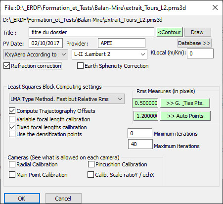
Choice of the method of calculation in Block according to the least squares - The method of GAUSS is rigorous. It leads to very important calculation times, proportional to the square of the number of unknowns. It is not very usable when the number of Images exceeds 1000.
- the method known as 'LMA' (Levenberg Marquardt Algorithm) calculates much faster. the calculation times are proportional to the number of unknowns
.- Less rigorous, it allows to reach results similar to the GAUSS method. On the other hand, it does not allow to obtain Rms in absolute mode.
For the moment, it does not allow calculations related to camera calibration. - The Automatic method chooses GAUSS if there are camera calibration calculations or if the number of Images is less than 100. Otherwise, it chooses LMA.
It is interesting to leave LMA for all the approximate calculations because it is faster, and to finalize with the GAUSS method.
Activates the calculation of trajectography offsets. Only the requested offsets (checked in the "Trajectography" page) will be taken into account
Calibrates the focal length of all cameras with a variable focal length (each Image has a different focal length).
See the camera page for the type of focal length associated with each camera.
Calibrates the focal length of all cameras with a fixed focal length to be recalculated.
Enter the densification points in all least squares compensation calculations (otherwise, the 'da123..' are not taken into account.
Minimum number of iterations and maximum number of iterations in a least squares calculation. The GAUSS method takes these parameters divided by 2.
Calibration request of the current camera. The main point and possibly the Y/X scale ratio of each pixel in the image. With the new cameras, this ratio is generally 1
Request the calculation of the radial and pincushion corrections.
Check that on each camera this option is possible. It is usually 1
1) Quick method for setting up images
- Open an empty Aerotriangulation file (when opening, do not put a file name or 'escape')
- Go directly to "Images" and drag your images into the list of Images (confirm the transformation of .JPG files into .tif)
- Go to "Autocorrelation" and click "Aero all Automatic".
- Possibly make a scaling by clicking on the button "Scaling"
- Heading "Models", create your models and double click on the desired model.
This method is expedient and only works for small projects that do not require precise calculations. The camera focal length values are extracted from the image files (provided they are tagged in the image). There is no camera calibration. In general, you have to go through the different phases described in the following chapters to get better results.
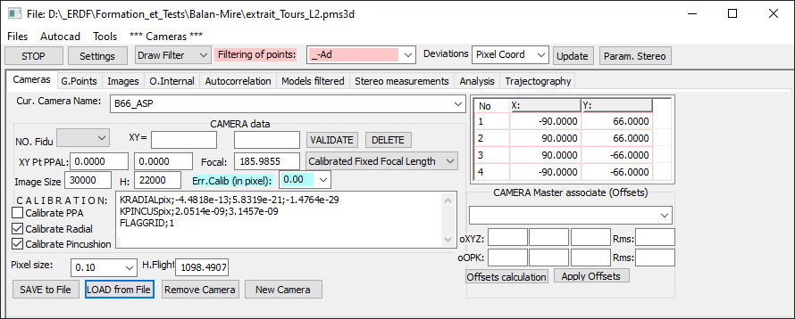
PMS3D can calculate with several cameras in the same file.
The coordinates of the fiducial points, the focal length and the flight height are defined.
This information can be saved in an ASCII file and reloaded later.
: Allows to choose the current camera from a list. This list contains the cameras of the site.
It is possible to insert other cameras by reloading a new one or by modifying the current one. (Change its NAME).
: Corresponds to the list of fiducial points. They are usually expressed in mm. The unit must be the same as the focal length.
In the case of digital cameras, the order of the points is as follows:
-Point 1 = Top-Left point of the Image.
-Point 2 = Top-Right point of the Image.
-Point 3 = Bottom-Right point of the Image.
-Point 4 = Bottom-Left point of the Image.
: Allows you to define the type of focal length for this camera.- This focal length can be fixed. In this case, calculation of this focal length is impossible. The Images related to this camera, will take this Focal length.
- This Focal length can be "to calibrate". The recalculation by the block compensation is possible. The Images related to this camera, will take this Focal length. To recalculate it en bloc, remember to validate the recalculation of focal lengths in the calculation parameters)
- This Focal length can be "Variable". The Images related to this camera will have a focal length independent of this camera. The block compensation of the variable focal lengths will update the focal lengths of each Image, without affecting that of this camera. The focal length of this camera is only used to provide an initial value for the Images.
: Defines the calibration elements that can be recalculated.
For example, to recalculate the PPA of this camera, you must check the corresponding box.
You must also check the PPA calculation in the general parameters of the block compensation ().
: Is an Editing Area, allowing to define a camera correction.
You can define a Radial correction as follows:
RADIALCOR;2.00;0.0378;0.0688;0.0934;0.1096;0.1145;0.1056;....
RADIALCOR >> Radial correction; 2.00
>> 2 mm steps. The correction at the center of the lens is always equal to 0.
0.0378 >> For a radius of 2mm, there is a correction of 0.0378mm or 37.8 microns (If the units of Images and focal length are expressed in mm).
0.0688 >> For a radius of 4mm, there is a correction of 0.0688mm.
So on for the following corrections.
You can define radial K and Pincushion correction coefficients as follows: - in mm (Image units)
KRADIALmm;-4.740900e-005;6.476800e-009;2.
017800e-011PINCUSmm;-1.238600e-005;4.847100e-007
- in Pixels (Image units)
KRADIALpix;-4.740900e-005;6.476800e-009;2.
017800e-011PINCUSpix;-1.238600e-005;4.
847100e-007FLAGGRID;1
- in units for single focal length (e.g. type PIX4D)
KRADIALp4d;-4.740900e-005;6.476800e-009;2.
017800e-011PINCUSp4d;-1.238600e-005;4.
847100e-007FLAGGRID;1
radial distortion correction
:DX = X*(K1*R^2 + K2*R^4 + K3*R^6 + K4...)
DY = Y*(K1*R^2 + K2*R^4 + K3*R^6 + K4...)
pincushion correction (weaker and not mandatory)DX = P1 *
2*X*Y + P2 * (R^2+2*X^2) + DY = P2 *
(R^2 + 2*Y^2 ) + P1 * 2*X*Y
with :
X,Y = X,Y "Raw" image brought back to the perspectival center; units in Pixels. Image to Terrain directionIf
FLAGGRID;1 then :
X,Y = X,Y "corrected" image brought back to the perspectival center; units in Pixels.
Direction Terrain towards ImageThis is
the mode of operation of the majority of the software.
R =SQRT (X*X + Y*Y
)R^2 = R to the power of 2
You can define a correction according to a Grid in the following way:
GRIDCOR;3;
5GRIDCOR01;-1.1,1.2;1.3,1.4;1.5,1.
6GRIDCOR02;-2.1,2.2;2.3,2.4;2.5,2.
6............
GRIDCOR05;-5.1,2.5;1.1,2.2;4.1,2.5
Explanation:
GRIDCOR;3;5 Correction according to Grid (in Pixels), defined on 3 columns and 5 Lines.
GRIDCOR01;-1.1,1.2;1.3,1.4;1.5,1.6 >> Corrections 1st Line (Y pixel=0). In Xpix=0, X correction = -1.1 and Y correction = 1.2. In X=X Image Size, X correction = 1.5 and Y correction = 1.6GRIDCOR05
;-5.1,5.2;1.1,2.2;4.1,2.5 >> Last Line Corrections (Y pixel=Height Image Size) In Xpix=0, X correction = -5.1 and Y correction = 5.2.....
Same principle for the intermediate lines.
The Corrections :
RADIALCOR and GRIDCOR are cumulative if they are both listed.
Warning: Whether in Radial or Grid mode, the corrections are made at the corners of each image tile, the interior is compensated proportionally.
If the corrections are very important, it is advised to reduce the size of the image tiles to keep a good precision.
With tiles of 128x128 pixels, radial corrections of several 1/10th of a mm are perfectly corrected
: Allows to save the values of the current camera or to insert a new one.
: Allows you to link this camera to a Master camera that must be included in this Field.
For example, the camera "LEICA CITYMAPPER" is a camera composed of 5 cameras welded together.
It is generally considered that the "Nadir" camera is the reference camera. The other cameras ("back", "front", "left", "right") are considered as cameras linked to this "Nadir" camera.
This could also apply to multiple cameras attached to a vehicle for example.
For the link to exist, the snapshots related to the master camera must exist in the project.
The snapshot "0025_back" will only be linked to the snapshot "0025_Nadir" if both snapshots exist in the PMS3D project.
However, it is possible to create a virtual snapshot of type "0025_InertialCenter" corresponding to an inertial center. The link
between the snapshots is made by the "TIME" field and if no value is available, by the proximity of the distance with a maximum of 10 meters.
Logically, the images to be linked were triggered at the same time to the nearest millisecond.
For each of these slave cameras, we must in the following fields, provide the elements, the transformation that allow to pass from the master camera to this slave camera.
To have these elements, the principle is to make an Aerotriangulation in block without these links between cameras and to calculate these elements by the buttons [Calculation Offsets] below.
: Displays the XYZ and Rms XYZ values of the offsets allowing the switch from the Master camera to the slave camera.
These coordinates correspond to the offsets of this slave camera in the master camera system.
The value of the Rms is the precision (the strength, the weight) of these offsets. A null or negative value invalidates the offsets. In the least squares, an equation is added to maintain these offset values.
It is important to understand that these offsets can vary from one photo to another. If between 2 cameras, there is 1 millisecond of delay on the Shoot of an image, we create a random XYZ OPK offset between the 2 Images
.
: Displays the OPK (Omega, Phi, Kappa) and Rms OPK values of the rotations allowing the switch from the Master camera to the slave camera.
The operation is similar to that of the XYZ offsets above.
: Allows the calculation of the XYZ and OPK, offsets based on the average of the offset on the whole set of Images.
At each shoot, we have a set of Images of the form "001_ClicheMaitre", "001_ClicheEsclave01", "001_ClicheEsclave02",.... then at the following shoot "002_ClicheMaitre", "002_ClicheEsclave01", "002_ClicheEsclave02",...
At each shoot, we have offsets "001_ClicheMaitre" with "001_ClicheEsclave01". The result of the XYZOPK offsets is the average of the offsets for all the shoots.
To calibrate these offsets, we make a mission that we calculate as independent cameras and once the block compensation is finished, we associate the Master camera with each slave. With this function we calculate the offsets. If we
receive a complete trajectography from a multi-camera "Citymapper", this function allows the calculation of offsets on the basis of this trajectography. This
function also allows to list the differences between the theoretical positions of the Images and their real positions (Excel table .csv) without any average calculation.
: Allows you to apply the current offsets to the trajectography or to the Images of the projectFor
example, if we have a trajectography of the "Master" Images, then we deduce the trajectography of the Images relative to the slave cameras.
In the same way, based on a block calculation of the "Master" Images, we can deduce the settings of the "Slave" Images
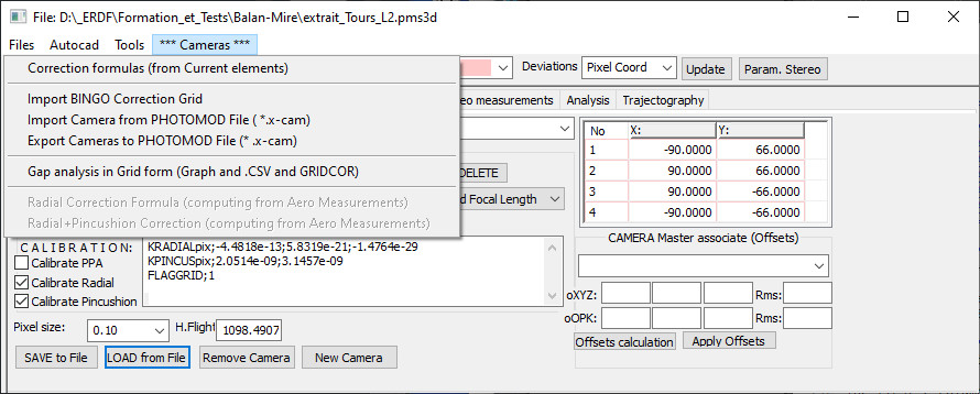
: This function transforms the current corrections into Formula mode.
For example if your current calibration is of the Form :
RADIALCOR;1.00;-0.0002;-0.0012;-0.0040;-0.0093;-0.0179;-0.0303;
This can be replaced by The Formula:
KRADIALpix;-3.4837e-009;1.0522e-016;4.
7762e-025KPINCUSpix;-1.2327e-008;-2.5220e-008
: Allows to import a Bingo type GRID calibration.
The data are of the form :
* Correction grid from BINGO's additional parameters for camera H3_35_11_05_22*
step width : 2*
x', y' min. and max. : -30 3040
.9 62.7 -30.0 -30.
040.0 62.9 -28.0 -30.
038.7 63.1 -26.0 -30.0.....
The first 2 columns correspond to the X and Y correction in Microns (value Images
)The 2 following ones are the coordinates X,Y Images of the corresponding point.
: Import and Export of the elements of this camera in a --.x-cam file, used by PHOTOMOD.
Only the KRADIAL, PINCUS and RADIALCOR corrections are imported and exported.
: This function is eliminated. It is integrated in the block calculation.
: This function is eliminated. It is integrated in the block calculation.
3) Import cue points if necessary.
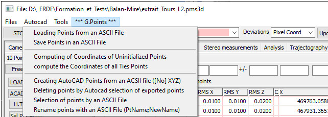
Buttons for Import, Export points in an ASCII file. In general, points are imported from an ASCII file of the form
:Point_Name, X, Y, Z, EmqX, EmqY, EmqZ.
Buttons ) to import points from an AUTOCAD selection set.
Buttons ) to eliminate unnecessary points (AutoPoints with less than 2 measurements).
Buttons ) Impose a Text Height when exporting these points to Autocad.
Menu ) Recalculates the least squares coordinates of the selected Ties Points according to the current settings of the Ties Points.
Menu ) works on a set of selected points. You can change their type but also export them or change their Emq.
Menu ) To create point entities in Autocad from an ASCII File. Interesting function for its efficiency in the case of dense pointsMenu
To import/export Aerotriangulation points in ASCCII or to Autocad.
Menu ) To delete points and associated measurements by Autocad selection.
Menu ) To delete relative coordinates and coordinates from block compensation.
This is useful when the calculation in blox diverges. Once these coordinates are deleted, the calculations can converge again.
The points must first be exported to Autocad. By graphical selection you can then eliminate the points that you think are wrong.
Menu To generate terrain sheets according to a model.
With these elements, an operator will be able to measure these points in the best conditions.
See an example of model (PMS3D\Modeles\Modele_Standard.html) to see how to adapt a model to your company.
Menu To rename the points. You can easily change or insert the 2nd character of the point
.
For more complex modifications, it is possible to write an "Autolisp" function of the form :
(defun c:PmsRenCli(cliName / newName)(setq newName (substr cliName 2))
)or to set a fixed length
(defun c:PmsRenPoint(sPtName / sPt newName)
(setq sPt (strcat "00000" (substr sPtName 2)))
(setq newName (strcat (substr sPtName 1 1) (substr sPt (- (strlen sPt)) 6)))))
Other models can be found in the file "PMS3D/DLL/PMS_LISP.LSP"
These import-export functions allow you to enter or modify points with the very powerful graphic editor of Autocad or by means of ASCII files.
It is also possible, when entering measurements (following steps), to provide a graphic point from Autocad as a set point. It will be given a chronological number
It is very interesting to finish with the Autocad export of all these set points that will allow us to find our way around; especially for the creation of models
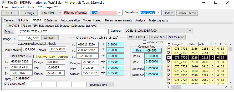
4) Images, parameters and processing.
Bar contains a quick summary of the functionality of the button or object under your cursor.
This is the most efficient way to find the function you need.
This quick help is implemented on the most important dialogs.
Button Assigns all of the following Rms values to the GPS CP data of all Images. Rms (Empty) or -2 values are not affected. An Rms value of -1 causes the CP GPS value to be invalidated.
Values These values are the current default Rmss that you can apply to GPS CPs if any. They are also taken when creating or importing new CP GPS.
Tag ( For aerial photos the angles are presented (and stored) according to PHI, Omega, Kappa in decimal degrees. In terrestrial, the angles of the form Bearing, Vertical angle and KAPPA=Camera rotation in Grades are more readable.
To associate a camera with the current Image. This is necessary in the case where there is a grid or radial camera correction.
In other cases, if there is no camera defined for this plate, the setting will be based on the current camera when calculating the internal orientations.
The focal length and the flight height are parameters linked to each Image.
Defines the offsets, in the camera system, of the lens center. Interesting in the case of terrestrial Images. See (CLI 03) for more information.
4.1) Create the Images by importing the images.
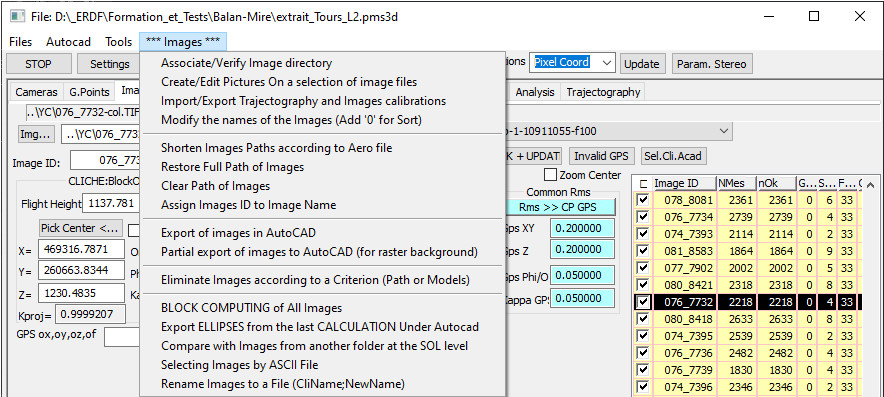
Menu When starting from an existing project containing images, this function allows you to associate a new directory for each image not found.
Menu To create snapshots by selecting images with the Windows Explorer.
It is also possible to drag this list of filesdirectly from thewindows Explorer to achieve the same result.
This is the method to be used as soon as the site is opened to create all the Images automatically.
By Selecting or Dragging files under Windows you import and create all your Images (Not set for the moment).
ADS80 mission case
You must drag the "---.SUP" files and not the "---.TIF" files.
You will then obtain directly called files ready to use.
You will only have to adjust the size of the models to have an automatic change of model adapted (see )
4.2) Import/Export the Trajectography (GPS points and angles) or the perspectival centers of the Images.
Menu To import/export a trajectography file (GPS points and angles) or the perspectival centers of the Images.
- Import/export of the setting elements and GPS elements of the Image centers Enter
You must define the order of the columns in your ASCII file by a sequence of letters separated by a separator character.
Each letter has a mnemonic meaning (N for Name, X for X, O for Omega, P for Phi K for Kappa, eO for Rms Omega).
To advance a column without taking it into account, add a ','.
For example ",N,,X" implies that you skip columns 1 and 3, X is in column 4.
Buttons You can import and export standard Image settings and GPS points.
The order of the angles is usually Omega, Phi, Kappa but on some analog devices or BINGO you can have the order Phi, Omega, Kappa.
Depending on the case you choose the desired units (degrees, grades or radians) and the direction of rotation.
In case the Rms eX, eY, eZ.. are not present in the import file, we will use the ones shown in this dialog box.
If you are lucky enough to have some settings at your disposal or GPS points of your camera centers, your Images are then almost set.
Remember to copy the XYZ and omega, phi and Kappa values of the GPS CPs to the perspectival centers of the Images before creating the models. In
this case, the automatic manufacturing function of the missing models will create all your models and you will not have to do the model creation step.
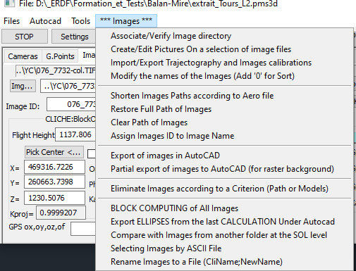
Menu To lengthen the number of Images by adding '0'.
In case you need more characters in the snapshot number, this function adds '0's to the snapshot number.
The Image number takes into account the last numeric characters of the Image name.
Menu Partial export of the snapshot frames.
Export the frame of the Images to Autocad. Unnecessary snapshots, which are completely covered by other snapshots, are not exported.
Menu Partial export of Image frames.
Export the frame of the Images to Autocad. Unnecessary snapshots, which are completely covered by other snapshots, are not sent.
new line 1
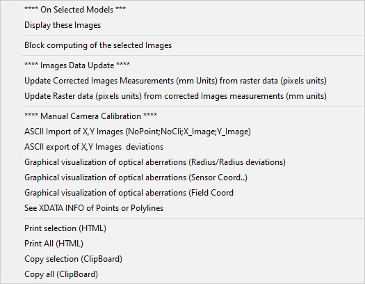
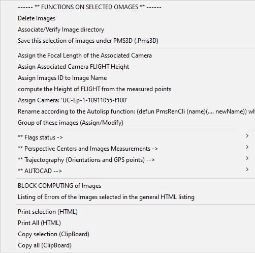
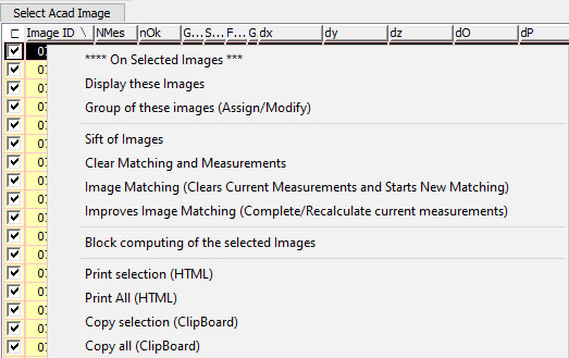
4.3) Processing menu Acting on selected Images (right click on Image list):
new line 2
new line 3
On an image selection set you can apply a series of functions.
In particular you can:
-Modify in series the camera focal length, the flight height, and
flight height, and reverse the axes of the Image (KAPPA + 180 degrees).
-Act on the Offsets (camera system) through the menu.
You can duplicate the offsets of a Image on a whole series or Validate the current non-zero offsets. This validation calculates a new perspectival center
corrected for offsets (ox,oy,oz and of) taking into account the current orientations and focal lengths of the Images. These notions of offsets allow, if you fix an adapted
support on a prism rod or on a tripod, to find precisely the perspectival center of the
precisely the perspectival center of the Image by knowing a point shifted in a constant way.
- Export and Import these Images under the graphic editor
Autocad. It is very interesting to be able to translate and rotate these Images in a very visual way under Autocad and to reimport the results. Everything is
reimported, including Phi, Omega and scale. For spatial alignment of the Images this feature is even indispensable.
- Lock/unlock snapshot orientation elements.
These features are especially useful when there are large errors in the
Aerotriangulation data, that the approximate orientation data are too bad and that the
are too bad and that the calculation in block becomes impossible (divergence of the
calculations). One then advances step by step until one highlights
the error. For example, we block the cliché centers at
± 1 meter and run
a calculation. We switch the Rms to 10 meters, recalculate. We end up releasing the
values with an Rms=-1.
Another method consists in launching the calculation on
some Images (right click on a selection of Images). This calculation being
correct, the orientation values of these images are blocked at Rms=0.
We recalculate with more images and we start again until we find the errors.
- Modify the Flags related to Images.
The different Images Flags are as follows:
- 0x01 : Approximate calculation of the executed point
- 0x02: Block calculation of the Dump executed
- 0x10: Relative orientation of Snapshot OK
- 0x20: Absolute Orientation of Snapshot OK
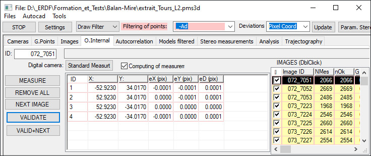
5) Enter the Internal orientations (Film photos).
Dialogue In the case of a digital camera, there is just to click on the button "Standard measurements".
You just have to apply this setting to all the Images related to this camera.
To do this, you need to define the coordinates (in snapshot coordinates:0,0
to the center of the image) of the fiduciary points of the camera in the following way:
No 1: Top Left (Pixels (0,0))
No 2: Top Right (Pixels (Xmax,0))
No 3: Bottom Right (Pixels (Xmax, Ymax))
No 4: Bottom Left (Pixels (0,Ymax))
Dialog If this box is checked, when you apply a new calibration, the cliché measurements are recalculated.
Thus, in the case of digital image, the Image measures are unchanged.
Dialogue This orientation parameter allows, in the case of terrestrial Images, to have only one camera for Images taken with the camera in vertical or horizontal mode.
camera for Images taken with the camera in vertical or horizontal mode.
To simplify things, when you take the Images, try to limit yourself to 2
positions. Horizontal corresponding to no rotation and vertical to a rotation
of 90 or 270 degrees.
Under no circumstances should the rotated images be modified by external software, otherwise you must create another camera adapted to this new rotation.
In the case of SCANNES, you must be careful to match the points you measure with those of the camera calibration.
By double clicking on a Image on the right, the image appears in a window.
You enter the fiduciary points of this first Image, you validate it, and you apply this calibration to all the other Images.
The first Image is set, the others are to be refined.
You put an adapted Zoom, the button VALIDATE+SUCCESS validates the measurements and displays the following image. At each click, you are presented with the next fiduciary point of the current Image.
If you have several cameras in this folder, then you go back to the "Cameras" tag to update the elements of the new camera and you continue your internal orientations.
The current camera is always taken as reference for the calculation of these internal orientations.
Don't forget to save the results of this step.
6) Automatic Aerotriangulation (Autocorrelation).
Autocorrelation allows to automate the calculation of the Aerotriangulation and to limit the
limit the manual entry of "Ties points". It consists of 3 main phases
- The creation of key point files. Each file has the same name as the image file and has the
extension ".sift".
Generally, only 10 percent of these keypoints will be associated with another image.
- For each pair of images, the search for identical key points (MATCHING) with beam calculation and elimination of
erroneous points.
- Filtering out the false points (about 40 percent) and iteratively calculating the aerotriangulation.
This phase is the most difficult because 40 percent of the correlated points are false, it is a lot and in some cases, if the approximate values of the calibration of a Image are false, we can find a
If the approximate values of the calibration of a Image are false, we can find a false calibration solution while keeping 50 percent of the points.
6.1) Creation of key points.
This functionality exists identically in the Image file preparation module (RASTERCONVERT).
RASTERCONVERT is faster and does not require a license.
This feature uses the graphic functions of the graphic card. The graphics card must be "OpenGL" compatible.
Parameters related to the creation of these key points.
The parameters are separated by a ';'. These parameters are documented in various bibliographies. Here is a link to one of them :
http://cs.unc.edu/~ccwu/siftgpu/manual.pdf .
Typical configurations can be predefined in the file "..\INI\PMS3D.DEF" heading "[SIFT_OPTIONS]".
The main parameters are as follows:
- -tc;80000 : Limit if possible the number of key points to 80000. We try to keep only the most interesting ones.
interesting ones.
- -no;-1 : Number of scale levels. xx=-1 >> only one level. It is interesting
interesting if the images have a similar scale. In this case the points are more precise.
- -fo;-1 : defines the first scale level (octave). In our case '-1' the first level corresponds to 2 times the size of the original pixel.
Image degradation level to calculate these key points.
- High: We calculate the key points on the undegraded image
- Medium: We calculate the key points on the image taking only one pixel out of 2. The main
interest is to decrease the computation time
- Low : We compute the key points on the image taking only one pixel out of 4. The main
interest is to decrease the calculation times
- Ultra Fast : We calculate the key points on the "thumbnail" image (sub image defined in AS03)
Thumbnail size (Thumbnail) Allowing fast matching calculations
We use this sub-image to test the possibility of correlating one image with another, to find possible image pairs and to calculate approximate beams.
This generates a significant gain in speed.
As a general rule, we set this value to 512 (512x512 pixels).
6.2) General principle of Matching and calculations.
In order to be able to process both 1Giga pixel images and images taken with consumer cameras, to manage several cameras, to take into account trajectography data and camera calibrations, not to limit the number of images, the all-or-nothing calculation option has not been retained.
The option taken is to be able at any time to calculate, stop or partially resume the setting of the project images.
The images already calculated are not resumed and are considered as correct. It is up to you to verify that these calculated images are indeed correct.
The new images try to be based on those already calculated.
An image is considered as calculated when its group is not null
.
We consider that the images of "group 1" have no link with those of the other groups
.
In principle, we start from the image that seems to us the best placed, we associate a 2nd which then takes the group of the 1st, then a third and so on.
About every 10 minutes, we save the results in a file: FileName_LastMatch.PMS3D.
In case of a crash, the recovery of this file gives you the last valid calculation
saved.
If at any time, the calculations diverge or the differences seem too large, the program stops automatically. You will have to analyze why, manually correct the problem and restart the rest of the calculations.
To add an image to the current group, the following calculations are performed:
- Search for images that have a relationship with this image.
- For each pair, beam calculation
- Addition of this image to the group and partial block calculation of the area where the image has been inserted
- Filtering of erroneous points and merging of points found in more than 2 images.
- Helmerth calculation if a new known point or a new image center with trajectography is
trajectography is added (this calculation is only executed if there are at least 3 known points or CP).
One of the main difficulties is to find, in front of a given state, the image best suited to the calibration.
In the case where we have a trajectory, even bad, the choice is made geographically, otherwise, we consider the alphabetical order of image names. If the last Image is "IMG008", we will start by trying to add the image "IMG009" or "IMG007".
The integration of a trajectography, even imprecise, is very favorable to the success of the calculations.
6.3) Preparation before the
Matching.
Before starting the Matching run, the following steps should be checked:
- <Cameras>: That the camera is the correct one and that it is calibrated if possible. That the focal length and flying height (distance camera<->object photographed) as well as the size in pixels of the image is well defined.
In the case of an uncalibrated camera, specify its inaccuracy in the box "Err.Calibre (in pixels)".
- <G.Points> : That the field points, as well as their Rmss if there are any, are correct and that the declared projection is the right one
- <Snapshots> : That the Snapshots are in the list. That for each Image, the associated camera, the focal length, the flight height are correct.
That the trajectography, if it exists is integrated and in particular that the Rms concerning this trajectography is correct. - <O.Internes> : That the internal orientations appear in the list. That for each Image, the associated camera, the focal length, the flight height are correct.
That the trajectography, if it exists is integrated and in particular that the Rmss concerning this trajectography are correct.
The trajectography can be imported from an ASCII file by the function "Images->Import/Export GPS Points and Images Settings"
If some of the data provided is wrong or inconsistent, the software will not be able to converge the Aerotriangulation calculations.
In particular, if the coordinates of the fixed points provided and measured are offset from the centers of Images provided by the trajectography, the orientation in Absolute of the Aerotriangulation will be impossible.
In this case, only the trajectography should be provided and an offset applied to these centers before entering the Terrain points.
6.4) Key point matching, filtering and calculations.
For files with more than 50 images, it is interesting to calculate a project sample. This makes it possible to define the starting images, to check the
parameters (Emq density etc...) and to start from data already set in absolute
data already set in absolute terms.
Once this has been done, even the automatic calculation will be based on these already calculated
already calculated and from the start will be calculated in absolute.
This process of partial calculation avoids calculations of several hours to finally not have the expected result.
To perform this partial calculation, 2 methods are possible:
- Start the project with a few Images (the best defined and allowing for an absolute setting), calculate it, then add the rest of the missing Images
- Use the Right Click on a selection of Images in the complete list, and ask for a MATCHING
Below are descriptions of the different options and buttons for Automatic Autocorrelation calculations.
<Density> Average number of points to keep per image. Let's consider this value equal to 800.
This option is used by the creation of key points; we consider that to guarantee 800 final points per image, 800 * 30 = 24000 key points are sufficient.
It is also used in the calculation and filtering phase. We try to keep an average of '800 points' per image.
The most interesting points remain in 'Auto points', the other pass in 'densification points'. In the calculations, only the AutoPoints are taken into account.
Mission type for these images.
In some cases, to make certain filtering decisions, it is interesting to know under what conditions the images were taken. For example, in the case of aerial Images, we can consider that all points distant from the camera of more than 2 times the average flight height or less than half a flight height are probably false.
Similarly, always in the case of vertical shooting, we limit the angles
omega and Phi.
For the moment, this option is only used to filter the points according to the flight height and for the
pre-positioning of the 1st Image (vertical or front).
The "3D Complex" type limits any filtering to the maximum. It can be interesting to visualize in stereo group photos in which there are
in which there are elements very close and others far away. This type of photos can be taken with a simple Smartphone or IPhone.
<Calculation Block> Launch or continue the Aerotriangulation calculation.
This option automates the complete Aerotriangulation calculation by linking the manual functions AC04 to AC07 described below and found on this same "DIALOG TAG Autocorrelation".
<MATCH> MATCHING, Key point association and cliché wedge element calculations.
This function is the heart of the calculation process. Cliché by cliché, it
This function is the heart of the calculation process. Plate by plate, it searches for all possible pairs with the plates already set, calculates an approximate position and integrates this plate in this group as a calculated plate.
The order of calculation of the Images is geographical if there is a trajectography, even imprecise. Otherwise, the order is alphabetical. The names of the Images have an important influence on the order of calculation.
Each time a new Image is added, the function tests whether it is possible to set the group in absolute. To do this, it needs at least 3 known points, either perspectival centers in the case where a
or known XYZ terrain points.
As soon as the absolute setting is done, the CP values and the measurements on the ground points are taken into account in all the calculations. In relative mode, they could not be taken into account because of the incompatibility of coordinate system.
In case of discrepancy of the least squares calculations or in case of impossibility to associate the current Image with already known
In case of divergence of the least squares calculations or in case of impossibility to associate the current Image with already known Images, we place this Image in a new group.
This new group then becomes the current group.
In case of stop of the calculations for non convergence of the calculations, it is necessary to try to find why the least squares diverge.
Either one or more plates are badly adjusted or have drifted progressively. In this case, it is necessary
In this case, you must temporarily eliminate these plates and force the calculation of other plates manually by using the Right-Click menu in the list of plates in this dialog.
Or the initial data are inconsistent. For example, the measured terrain points are offset from the trajectography or simply an error in the point number. Simply eliminate this point or the measurements on this point and restart the calculation en bloc
.
Or it is not possible to correctly integrate the current Image into the already calculated set.
Then the valid overlap area (where there are AutoPoints) is too small or a combination of circumstances means that false Autocorrelation points have not been detected and appear in the calculations. This can happen at the end of a band or during a band change for example. In this case, destroy the measurements on this plate
and impose the calculation of another or a series of better placed images
<Match Improves> MATCHING, from practically called Images, to improve results.
This function is similar to the previous one.
The fact that the position of each Image is known precisely, simplifies the function. Therefore, we test only the neighboring Images, we do not redo the matching between 2 Images if there are
enough points connecting them.
To launch this function, the parallax must not exceed 10 pixels.
This function is very interesting for the recovery of areas where there is still some parallax.
It can also be used if you have a very precise trajecto.
<Merge Points> Merge points between Images.
Globally, for each computed snapshot, this function merges the identical points. When a location in an image is
correlated on several images with a different No, they are grouped under the same No.
Before doing this operation, we check that the differences are within the tolerances.
This function can be launched at any time.
<Rms> filter; Filtering and removing out-of-tolerance points.
You are asked to provide a number of Rms overshoots. It does not ask for an absolute distance such as
We do not ask for an absolute distance such as meters, snapshot units or a number of pixels because each measurement can have different sources and therefore different accuracies.
For example, we can consider that the measurement of a GPoint is done at +- 0.3 pixel while an
AutoPoints is rather +- 1 Pixel. In these cases 3 times the tolerance corresponds to a deviation of 0.9 pixel for a manual measurement and 3 pixels for an AutoPoint, which corresponds to a deviation of 0.1 pixel for a GPoint.
Autocorrelation, which actually corresponds to reality.
For the Automatic correlation, we set the Rms of the measurements to 1 pixel if the precision is "High", 4 Pixels if the precision option is "Low"
As we can mix cameras with different accuracies, we are obliged to reason in terms of the number of Rms overruns and not in terms of tolerance in the sense of absolute deviation.
This function takes into account the requested point density value. It tests the density of AutoPoints on each plate and by geographical location to try to approach the number of points requested per plate.
The most interesting points remain in "AutoPoints" and will be used for the calculation, the others go to "densification Points" and remain available in case of later need or change of the "density" variable.
This function can be executed at any time
<Block> calculation; Filtering and elimination of out of tolerance points
Launches a Block calculation of all the Images with enough measurements. The calculation is performed even if no absolute orientation data is provided.
This function can be executed at any time
<Helmerth 3D> Absolute calibration of current group
This function is built into the Matching.
However, you can restart this function at any time. It is interesting in the case where you have
This is useful if you have moved your trajectory or terrain points for example.
The same applies in the case of a discrepancy in the calculations, in the case where an absolute setting has been made on nearby points and that a few dozen Images later a new terrain point enters in compensation. The effect of the lever arm is that the approximate values of this point are too far from reality. A manual Helmerth3d restores the situation.
You can also use it to control "Ground Points". You will then see,
You can also use it to check "Ground Points". You will then see, thanks to the Helmerth deviation table, that the deviations on this point are important and you can remove it from the calculations.
This function can be executed at any time. Depending on the Helmerth deviation, you can validate it or not.
<Scaling> Scaling the current group
You have a project of some independent photos and you just want to scale it. With this function, you associate a distance measured on the photos with a distance on the ground
.
Before running this function, your project must be calculated.
This function can be executed at any time
<Maj.Statistics> Updated the Quality Statistics related to this Aerotriangulation.
We update the table relating to Images, located on the right. [Update Statistics] button in the Autocorrelation page to update.
- Respectively, relative to this
Snapshot: Number of measurements, Number of Valid measurements.
- Flag +1: This snapshot is calculated; +10: The relative orientation is Valid; +0x20: The Absolute orientation is Valid..
- If there is a trajectography, the deviations found are found here. Abnormal deviations point to doubts about the timing of the Images involved.
- Number of snapshots attached to this snapshot by Matching. A snapshot is counted if it has at least 5% of the total measurements.
- Number of measurements on a Ground Point (Stereopreparation Point).
- For [X 0] we have the number of measurements in correspondence with Images located to the right of this image (X0). Same principle for X<0,Y>0 and Y
<0.br>
- Percentage of image area covered by measurements.
- Percentage of measurements falling within tolerances
- Confidence index (from 0 to 10). It depends on the
attachment of this snapshot to the neighborhood, its matched area and the deviations on its measurements. Percentage of measurements within tolerance. A plate at the corner of the file will therefore have a bad index while it is not bad.
- The more '*'s there are, the more doubt there is about this calibration. The number of stars is related to the confidence index..
lt; Ctrl.Graphique Graphic display of the diagram of this Aerotriangulation.
6.5) Right Click menu on selection of images.
<Assign/Modify the group of these snapshots>
Allows you to modify the group of Snapshots. Just be aware that two Images in different groups are considered to have no relationship.
This can be used to temporarily isolate some Images from the list of Images to MATCH.
<SIFT of Images>
This is the "SIFT" function seen above but on a selection of Images.
<Clear Matching and Measurements>
All autocorrelation measurements on the selected Images are cleared. The group as well as the Matching Flags are set to zero.
The measurements on the TPoint and the GPoints are kept as is.
<MATCH Images>
This is the "MATCH" function seen above but on a selection of Images.
6.6) Ground point measurement.
If the Images are not yet set in Absolute mode, you should proceed as
following manner:
- Select 3 or 4 of the best identified points, using the
Stereo measurements or, in the Trajectography dialog, the
Right Click functionality on a point -> "Manual Measurement (For Cliché/Modele not set to Absolute)"
A minimum of 2 measurements in mono or one in stereo are required on each of these points - Run the <Helmerth3D> from the <Autocorrelation>
- Relay a Block calculation
- Get the other points by using right click on a series of points in the in the <Trajectography> dialog, "Measure selected points in Stereo/Mono". See the trajectography documentation for more information.
- Running a calculation in Block
6.7) Checking and improving results.
It is then possible to eliminate the completely wrong measurements and put back some that seem useful.
A new block compensation is then started, with or without recalculation of the offset.
It is also possible to request a camera calibration based on the current Aerotriangulation measurements. See the documentation for the dialog <Cameras>
The Point Filtering function (Emq Filter) is very handy and can be called at any time to bring measurements back into tolerance and remove others that have become out of tolerance
Another interesting function is found in the Dialogue <G.Points>
By right clicking on a series of points, you have the possibility to recalculate these points, even taking into account invalid measurements. In fact, some deviations in the Analysis module are high, simply because the point in question was not recalculated in the block calculation (not enough measurements or considered false).
In the same dialog box, the button "Purge Points" allows the deletion of
deletion of useless points because they have no measurements.
7) Creation of Models (pair of stereoscopic images).
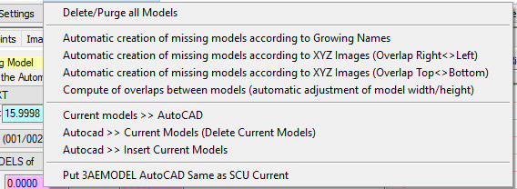
Menu Creates all the missing models in an Automatic way.
It relies on the alphabetical order of the Images to constitute the models (CLI01 with CLI02...).
For air flights, this is generally the case. In the case of Images named CLI_9,CLI_10... it will not work correctly.
At the end of the creation, a recalculation of the overlap is executed
Menu Creates all the missing patterns Automatically according to their position (Graphical Analysis).
Depending on whether the camera is at 90 degrees or not (Portrait Mode or Landscape Mode), or the definition of the trust points, there are 2 possibilities.
In general, if the Images appear Vertical the Right/Left solution is the right one. If they appear Horizontal it is Up/Down the solution.
If there are some in all the directions, it is necessary to create the 2 possibilities
Menu Recalculation of overlaps between Models.
The recalculation of the position of these models, corresponds to a recalculation of the model from the information clichés.
The width and height of overlap to provide is expressed in field units (usually in meters).
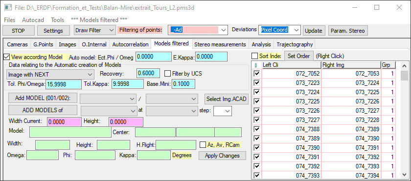
You have to create your models, generally by flight band.
Depending on the direction of flight and the future orientation of your model (due north when possible and not due south), you give the number of the leftmost Image of your band and the one of the rightmost Image (In the case of flight
(In the case of return flights, the highest number will be on the left).
When you load a model, the view will conform to the Phi/Omega and Kappa angles of the
model if checked.
In the case of not checked, we will try to keep the orientations of the current view
current view; There will then be a check that the tolerances related to the Z-axis and Kappa orientation are respected (DM 10).
For aerial photos the angles are presented (and stored) according to PHI, Omega, Kappa in decimal degrees. In terrestrial, angles of the form Bearing, Vertical Angle and KAPPA=Camera Rotation in Grades are more readable.
When in Automatic model, the change of
model checks that the verticality and orientation deviation (DM 03) are met.
If they are not, we move on to the next model test
According to the overlap between Images in the direction of flight, to have a correct base to height ratio we can no longer
to have a correct base/height ratio, it is no longer possible to count a 'ShotX/Image X+1' model.
This option allows to impose 'CLI_X/CLI_X+2' or 'CLI_X/CLI_X+3'... . The 'Auto Next Image' mode takes into account the desired overlap to find the best solution.
best solution.
This option has a direct impact on the accuracy of future XYZ measurements.
Defines the desired overlap rate between 2 Images of a Model.
This Value is used by the creation of the models according to the graphic position and also according to the alphabetical order
If the associated snapshot choice is Automatic (DM 03)
Only take into account Images that respect the current UCS
This is interesting in the case of facade for example. If our current is in the plane of a
building facade, only the Images concerning this facade will be used to generate the models
Defines the Width and Height of the models to be created (X Scale and Y Scale of INSERT
AutoCAD).
Allows you to define a particular order of the list of models. This is interesting
to change the model in terrestrial Photo.
In a plllanplaneiven Image, Automatic Image switching works well, even in spatial mode, but when you need to switch from one building face to another
face, the solution is to launch the 'PMS_CURMODEL' command (found in the PMS3D palette in Model+ and Model-). This command passes from the current model to the previous or next model by respecting
the order defined by the Indexes.
With a Right click, a menu allowing to export, delete or modify
delete or modify values will act on the selected models.
Allows you to add all the models of a band by defining only the 1st and last snapshot of the band.
Allows the addition of a single Model.
You will be asked to click, in Autocad the center of the Left Image (At ground level or the object being photographed), the center of the rightmost Image and a third point (or option H for Horizontal plane= Aerial PV or V for Vertical plane
You validate the recalculation of the perspectival centers of the Images. See below for the verification of the generated models.
Displaying and editing data related to the
current model. The modification is effective only after validation (DM 11)
Definition of tolerances that define whether or not to reorient the current view when loading a model. If the tolerances are exceeded, the view is oriented according to the snapshots. In the case of automatic model calculation, these values are also taken into account. The mini base avoids, in terrestrial mode, the mounting of a model on 2 Images with the same Perspective Center.
Mandatory validation for the above manual modifications to be taken into account.
Verification of generated templates
You must check the validity of the generated templates in 2 ways before proceeding to the next step:
1) By double clicking on a template (right) the template will be displayed in a window.
You check that the overlapping area is conform (Image "6915" on the left and "6914" on the right), that the name of the view is "6915/6914" and not "6914/6915".
If this is not the case, you can correct it by adding 180 degrees to the Kappa of the concerned Images (Right click menu on Image List, Dialogue "Images" , or by reversing the names of the first and last Image and repeating the previous operation or by rotating the current Autocad view by 180 degrees.
You can also check the coordinates of your fiducial points. If their direction is reversed, you have an inversion function in the "O.Internals" section. This last solution should be used with caution.
2) Menu to export the Models to Autocad. You can then check their size and relative positions.
You can use Autocad functions to manipulate these INSERT "AERMODEL", apply translations, rotations, scale changes, Change of Normal coordinate system changes, size changes.
When all the models have an overlay area that you like, you can then re-import them to validate these graphical changes.
3)Menu To Put the normals of the
models identical to the Current UCS of Autocad (by graphic selection).
Checking the consistency of the Perspective Centers of your Images.
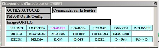
The LOAD/INS function of the palette allows you to load the images related to
these Images.
This way, you can visually check the consistency of your settings (verification
that there is no error of rotation of 180 degrees for example).
Notes:
These import/export functions for points, snapshots, GPS CPs and models in
models in Autocad can be used at any time.
This is a very visual way to check a snapshot state, or apply transformations to aerotriangulation the same way you would apply it to any other Autocad entity, there is no difference.
8) Enter measurements on models in stereo.
nbsp;
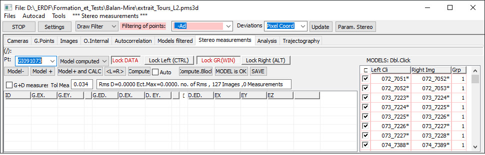
By double clicking on the name of the desired model on the right, the stereo image is displayed.
To start the input of one or more points, in an Automatic or No way. Before entering, be sure to check the My 02
option.
Be aware that the first letter of a point name conforms to the following conventions:
N >> New or New Point. This point is only in this template for now. It will change to a T as soon as this template is validated.
T >> Transfer point already measured in other model(s). Normally we don't have to change the existing measurements but only complete those related to the unmeasured plate.
Z >> Point only known in Z.
P >> Point only known in XY.
Any other letter considers the point to be a known terrain point in XYZ (unless the emqs say otherwise: emqX=-1 >> X of the unknown point).
Defines whether Images are calculated or Not. Only Images marked as not calculated will be compensated or not blocked.
If you have "Right not calculated" this means that you consider the Left snapshot to be calculated and therefore not editable, so the Right snapshot will rely on these values of XYZ and Phi, Omega and Kappa from the left to place itself.
Blocks (lock) or releases the cliché movements. The CTRL,WIN and ALT keys have the same effect.
To move to the next or previous model.
To run a model calculation (independent model; not in block).
If Auto is checked, Then, there is an automatic calculation at each point entered.
Block calculation of the whole project. Snapshots without measurements are automatically excluded.
Model validation. The 'N*' points become 'T*'=Ties points which will be, for any independent model calculation, considered as
independent model, considered as Fixed points. Do not forget this step as soon as a model is entered and no longer contains errors.
Procedure for entering measurements:
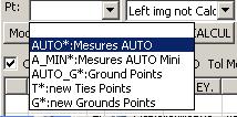
In the drop-down menu of point names validate AUTO*
. The system will automatically move as close as possible to the points to be measured. You have a pedal (or button) to block
to lock one Image in relation to the other, another to launch the Zoom=2, and a third to validate the point.
a third to validate the point. The space bar skips the measurement of an unmeasurable or useless point.
The order, position and number of connection points to be entered can be configured
and defined in the configuration file "PMS3D.INI" here is this line:
Posit of NewTiesPt in Auto mode (FX,/FY,>>Tol Rech X/Y ; N,PosX,PosY >>New Point ; T,PosX,PosY >>New Pt (search on TiesPts)
NEW_TP=FX,0.15!FY,0.15!T,0.1,0.1!T,0.1,0.9!T,0.5,0.5!T,0.9,0.1!T,0.9,0.9!T,0.5,0.1!T,0.5,0.9!T,0.1,0.5!T,0.9,0.5
We work in an Image coordinate system. The point of coordinates 0,0 is at the top left of the image
The point with coordinates 0,0 is at the top left of the image, the point with coordinates 1,1 is at the bottom right.
FX,0.15 defines a search area of +-0.15 * Image width.
The letter T means that if there is already a Ties point at a location, we will use this point as the orientation point.
If you measure the point next to it because it is not possible to point it, then you will measure a New Point when you unlock the plate.
Menu is Similar to the previous function except that the number of
Ties points proposed is reduced.
Often only 2 axis points are put per Image. This function is suitable for missions with a trajectography.
In PMS3D.INI the corresponding variable is : NEW_TPMINI=FX,0.15!FY,0.15!T,0.5,0.1!T,0.5,0.9
Menu Automatically balances the Grounds Points of the
model not measured. Similar to the previous function except that there is no testing or creation of Ties points.
Once the first 6 points are measured, you normally have stereo.
Automatically, you will be asked for the score of all the transfer points and field points that can be measured on this model.
The hardest part is to start and measure the first 2 or 3 points
The hardest part is getting started and measuring the first 2 or 3 field points. You will be moving by sight, from model to model until you have measured these first 3 points. The measurements of 2 points in XYZ, of a third in Z are
third in Z are sufficient to authorize the first calculation in block. It is sometimes
sometimes interesting to create a temporary point in Z (it will be transformed into a Tpoint later on), just to allow the block calculation.
You do not have to start the measurements with the model at the end of the strip.
It is more interesting to start with the model with the most known points.
As soon as a new point is measured, the independent model calculation is executed. In this mode of calculation of independent models (contrary to the block calculation),
the T points are considered as fixed points, only the N points are recalculated.
Don't hesitate to save or "save as" at each interesting step of the validated measurements.
All this seems complicated but don't panic. On the practical side, with practice,
it takes 1 to 3 minutes per Image:
I launch AUTO measurement.
I locate a point, pedal 'zoom*2', pedal 'unlock', I point finely with my
my cranks, 'pick point' pedal. I mark a point, .......... (for the 6 points of wedges).
I finely point the missing measure on a Image of the T point already measured on the other
the other, pedal 'pick point'...... For all the T points measured on the neighboring plates.
I refine the pointing for any proposed terrain point, pedal 'pick point'.
I restart Measure AUTO and complete any missing measurements.
I check the deviations.
I check the differences.
If I have at least three known points, I calculate in block:Mes 06
, I check the overall Emq, then validate the model ("MODEL is OK" Mes 07) and I save
("SAVE").
The checkmark "Draw
"allows you to display the points, measurements and deviations in the
stereo window.
I move on to the next model. So on.
Menu New Ties points manually:
In a loop you are offered a new free New point and asked to point it wherever you want.
Menu New Ground points manually:
In a loop you are offered a new free G point. You are asked for its graphic position in Autocad (CAD window) and then you are asked to point it on the stereo model.
Menu bar relating to the entry of measurements:
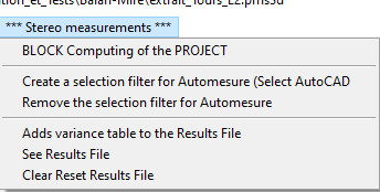
Menu To start the Project Block calculation.
Menu To Filter the points to be measured. Useful in land mode when entering
building facade.
This filtering avoids having in the list or in automatic measurement, all the points that are part of the
opposite to the one you are measuring.
To activate this filtering, you must export the points to Autocad and in top view, select the points relative to the current facade using this function.
to the current facade with this function.
Menu To remove the filtering activated above.
Menu Adds information about this model to the
template to the current results file (.HTML File).
Menu Displays the results file filled by the previous function (MB 04).
Menu Clears the current results file.
Note:
It is possible to display as many models as you wish.
Activating a window (by simple click), makes the table conform to it. The table reflects the data of the active window. However, it is necessary to be well
However, you need to be well organized to work on 4 or 5 windows at the same time.
The multi-window feature is especially useful for finding transfer points between bands.
When you click on a line in the table, a zoom is made on this point and, if it is a Ground point, the movements are blocked. If you want to
If you want to measure it again, either deactivate the "lock data" button or delete the measurement(s) already taken.
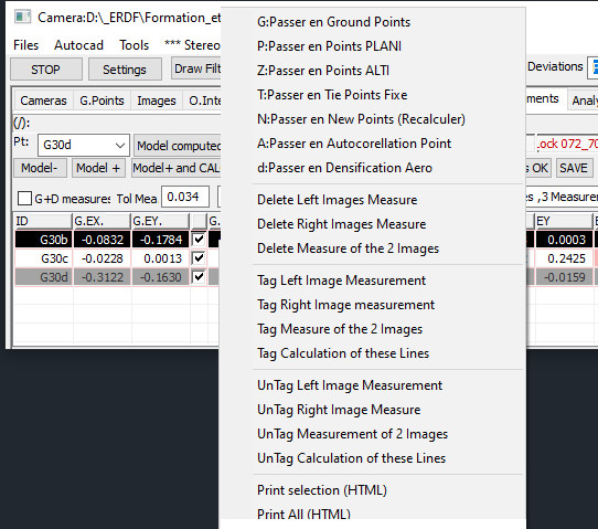
Right-clicking on one or more rows of the table offers the following features:
The right click on one or more lines of the snapshot table offers the following functionalities:
9) Files delivered with a Trajectography.
The aerial Images are now digital.
The GPS coordinates as well as the tilts of the Images are also provided.
In these cases, the Aerotriangulation calculations are very simplified.
You need to start by importing the data provided to you. Perform the following steps:
All of this takes little time and if your provider has provided you with excellent data, and you don't see any discrepancies on any ground points you know about, your
Aerotriangulation is complete.
Unfortunately, not everything is so simple and often you find unacceptable deviations.
The tools described below have been developed to improve results by correcting certain imperfections (material offsets or scales).
The principle is to measure additional data in the most efficient way possible.
There is no one rule that applies to all cases and you need to think about the best way to
think about the best method to correct deviations with the least amount of input.
Please note that it is not advisable, or even impossible, to check the calculation of all offsets; some are similar.
offsets; some are similar.
For example, recalculating the Roll, Pitch (TR 07) at the same time as the dX Cam and
dY Cam (TR 08) will probably result in a singular matrix; unless you have
measured points at very different altitudes (very rough terrain) or
flight heights that vary significantly.
Indeed, in the aircraft system, at the same flight height, an offset_Pitch is
similar to a dX_Cam.
We have the similarity relation dX_Cam.=Flight_height * sine(offset_Pitch).
To simplify, we check only one color and, if we have terrain points, we add the Cyan=Offset X, Y and Z GPS.
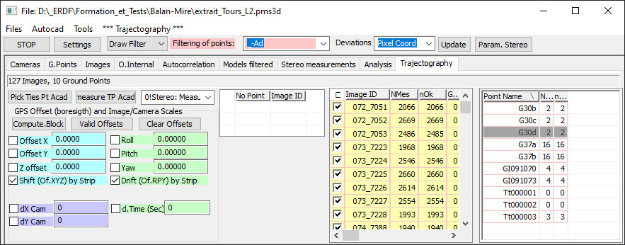
Below is a description of the features of this dialog box "TRAJECTOGRAPHY"
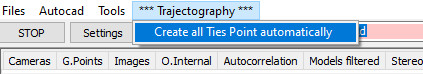
Menu : Create TP AUTO :
To automatically create new Ties points. For each Image, we try to place a low point and a high point in the X axis and if requested, a point in the center.
Before creating these points, we check that there is not already one. There is a possibility to put only one point every 2 or 3 Images in the X axis.
It is about providing the tools to correct the possible systematic errors of the trajectography (data
from the aircraft's inertial units)
You also have here all the tools to measure the ground points of
stereo preparation or possible Ties Points that you find interesting
For a correction value to be taken into account, the corresponding [check mark] must be active.
In order for a correction value to enter the block compensation and be recalculated, the corresponding [check mark] must be active and also, in the Aero settings, the [recalculation of Trajecto Offsets] must be active.
For offsets related to XYZ and Omega,Phi,Kappa, you have the choice between a single correction for the whole file or a no-band correction
Buttons
to enter XYZ points in autocad and then measure them in stereo on the Images. With the
automatic correlation, this function loses its interest.
The [Pick Ties Point] button allows you to place Ties Points at the most interesting places (where they touch the most images).
You can then, thanks to the button
You can then, thanks to the [Measure TP ACAD] button, measure in series all these points on the images.
List of Images. '*' so stalled. Right click for menu of functions relating to Snapshots; double Click to display the Snapshot.
List of points measured or to be measured. In parenthesis is the number of measurements made on this point. Right click for menu of functions related to the points.
To select a Image in relation to a point, we check that this point is within 20 pixels of the edge
In some cases, it is interesting to increase this value by the command "PMS_PCLICHES" which allows to redefine this value (in X and Y).
Thus, during automatic measurements, we can eliminate points located too close to the edge of the images
Buttons&Combobox :
Pick Ties Pt ACAD. : To interactively enter in AutoCAD new points. Remember to put a correct Z or failing that a Zul (command:
Elevation).
A good solution is to open a stereo window in automatic Image change mode, and place these points almost permanently.
Thus
the following measurements can be made directly with the maximum zoom.
Remember to put a correct Z or, failing that, a Zul (command: elevation).
ACAD TP Measurement. : To measure a series of points that must be selected in Autocad. These points can come from the above function or from an Autocad export.
For each selected point, a model is proposed. The left cliché corresponds to the most favorable cliché (point as central as possible and measurement
already taken if possible). The other Images concerned will scroll on the right.
The option to measure in stereo was taken because it ensures a better precision of the measurements and avoids pointing the same point in different places.
Moreover, this option allows to measure in places where there are no characteristic objects.
For each point, all the Images are scrolled. A list of Images containing this point is created. The model cli1/cli2 is then presented, followed by cli1/cli3 etc...
In this mode, the arrows on the numeric keypad have the following functions:
Pick the point (or pedal 1): Record the measurement on that point. If it is a TP, then those coordinates are changed.
Spacebar: Skips the bar. Moves to the next right Image or if last, moves to the next point.
Right Arrow: Left snapshot retained, Next right snapshot (looped).
Left Arrow: Right Image retained, Next Left Image (looped).
Down Arrow (or Pedal 2): Locks/unlocks Image movement (looping)
Up Arrow: Skips to the next point or ends the function if no more points.
This function is interesting to measure points of connection between bands because we create a stereo with Images of several bands.
Combo Options: You have a filter option to offer only new measurements.
The 'MONO Measurements' options allow you to measure points in mono mode. Photogrammeters usually prefer stereo mode, but
sometimes, to calibrate a camera, this 'MONO' mode is interesting.
Buttons :
[CALC.BLOCK]: Standard block calculation of the project according to least squares.
In order for the offsets to be recalculated in block, you must not forget to check the []Recalculate Trajecto Offsets
in the Aerotriangulation parameters.
If not, the offsets values will be taken into account but will remain unchanged.
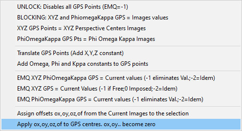
[Valid Offsets]: The values appearing in the "Edit boxes" correct the trajectory values (XYZ and GPS OPK shown on each Image).
With the current offset offsets corrections applied, they drop to Zero. You can then export this new trajectory corrected of any systematic
systematic errors.
[Clear Offsets]: To zero out all current
current offsets.
Options to process translation corrections in XYZ
of GPS (Geographic System) points. This option can only be used if you have
have measured at least one known point on the ground. Otherwise, you have a
singular matrix.
Options to process the corrections of
boresight corrections from the
inertial unit (IMU). This boresight consists in finding the offsets of Yaw, Pitch and Roll (respectively Kappa, Phi, Omega) to correct the IMU. Indeed, these angle values drift in time. The raw values are wrong.
Systematically, a correction constant must be added to them.
The boresight calculation used for your project must be recent and accurate. The quality of the offset values and therefore the trajectography depend on it.
It is advisable in any case to redo this boresight calculation in order to refine it.
Options : Processing of GPS offset corrections (GPS and inertial
inertial) by bands.
It is the same corrections as for the previous options 6 and 7, except that we have a different set of corrections for each flight band.
In practice, the [Shift (XYZ GPS Offsets) per band] option should not be used; this instrument already provides absolute coordinates.
This instrument already provides absolute coordinates.
In fact, the GPS measurements in the aircraft should be without offset or with a single general offset for the site that would depend on the pivot.
On the other hand, the option [Drift (OPK Offsets) by band] is very interesting.
Indeed, the inertial unit which provides these angles shifts and it is not rare that between two bands, the shift is important.
It is often when the aircraft turns around that this shift appears
Options to process GPS<->Camera offset corrections in the Aircraft system. The offset measurements of
the position of the GPS antenna with respect to the perspectival center of the camera made by the aircraft manufacturer are generally accurate. It is therefore rare to have to use
It is therefore rare to have to use this option, except possibly in the case of ground Images.
Options to calculate and process the phase shift between the GPS clock and the Top of the
camera. It happens that on some drones, equipped with a GPS with an accuracy of a few centimeters, the top Photo is shifted by a few milliseconds compared to what
from what is recorded in the trajectography file. This option allows you to correct this clock shift. If this value is constant on a given
material, it is interesting to apply this known and systematic correction from the start without the need to
necessary to integrate it in the
least squares calculation. For professional cameras such as the UltraCam for example, this option is unnecessary, these
inertial systems of very high quality have already made this correction.
List of the last 8 measurements. It allows you to follow the measurements you have just made and eventually
to devaluate or delete them in case of error of pointing.
Practical example of 3 bands of 10 Images (school case that we complicate for the demonstration):
- Import of the file (Images, trajectography and field points) and
preparation (Internal orientations, models etc...)
- Set Rms Cp GPS to 0.03 in XY, 0.04 in Z, 0.002 for angles; Rms
measurements of about 0.001 (1 micron) depending on the camera.
- Capture inter-band link points and field points.
(, functions).
- We consider 2 blocks. Block 1 = 6 Images on 2 strips (the first 3 + the other 3 corresponding to the bottom strip; block 2= last 6 on 2 strips.
- Enter Ties points on Blocks 1 and 2 below.
- Calculation of Offsets , ,
XYZ Row, Pitch, Yaw on block 1, then on block 2 and compare. If there is little difference then calculate the whole file.
- Apply the interpolated offsets in proportion to the bands (or
application of the average on all the Images).
- Control the results ;
- If bad, try the pattern blocking method:
- Rms Blocking of 0.01 in XYZ and 0.001 for Angles (Options )
- Rms CP GPS set to 1.0 in XYZ and 0.5 in Omega, Phi, Kappa to free up perspectival centers that are in doubt (See Images).
Caution: in the case of a single strip (or
several parallel bands flown in the same direction) with small gradients, the calculation of XYZ and Row, Pitch and Yaw offsets may result in
a singular matrix. In this case, just use Z and Row, Pitch and Yaw.
In the same way it is not recommended to calculate XYZ Offsets if you have not measured any points on the ground.
Translated with www.DeepL.com/Translator (free version)
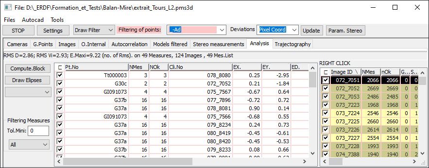
10) Analysis of results and correction of errors.
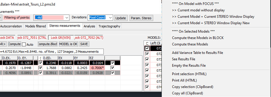
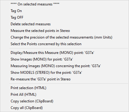
Right click menus on the Measures:
Right click menus on the Images:
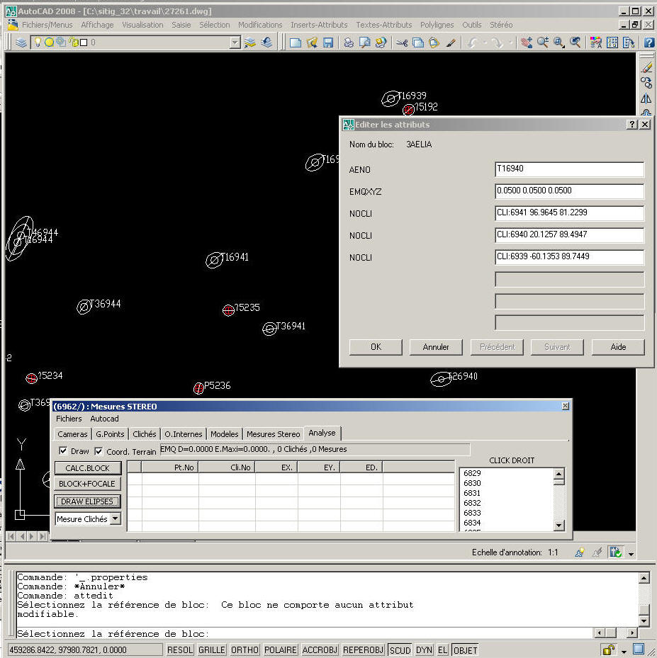
The middle table shows the measurements for the selected images on the right.
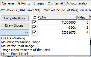
You can choose the desired effect by double-clicking on a line of the middle table
You choose the desired effect by double-clicking on a line of the middle table (in general you choose "Measure Point snapshots").
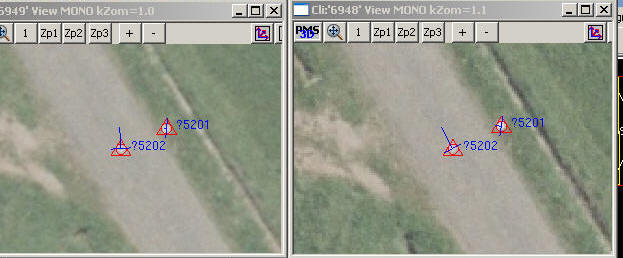
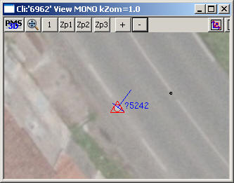
This means that a double click on the line of the point '?5202' leads to
the display of 2 Images, zoomed on this point ?5202 ready to receive a new
point.
Translated with www.DeepL.com/Translator (free version)
Donc ceci:
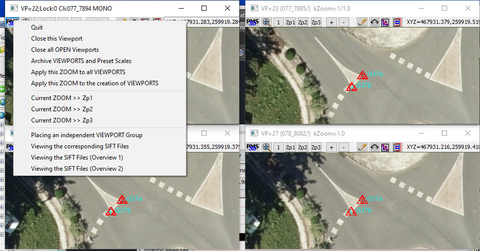
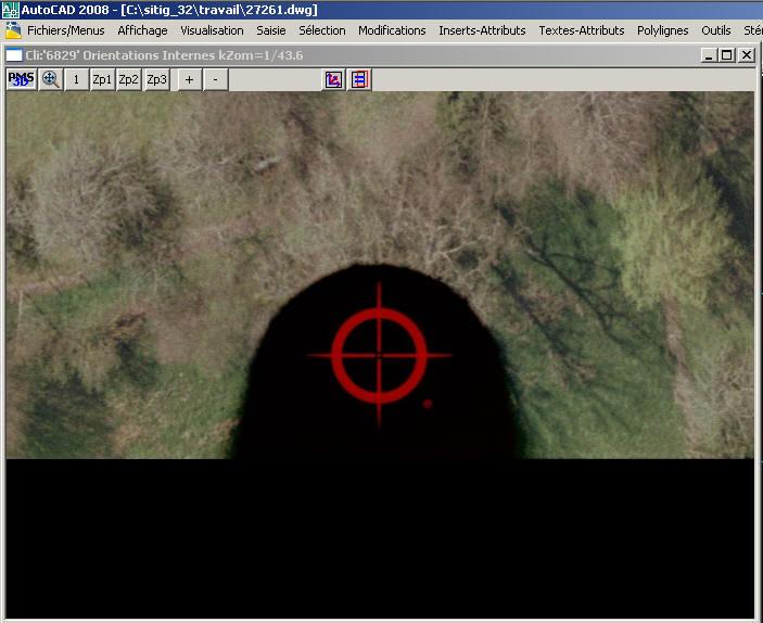
You define/archive your preferred window positions and zooms by
click on the "PMS3D" button:
For large deviations, this gives the following images (the 1st one with
the error and the 2nd one after the click).
The Bollar = field position, the long line = deviation and direction amplified by 50, the cross = real position.
Export visualization of the results.
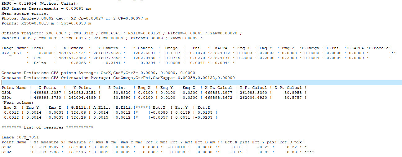
Here is a sample of the listing for the block compensation:
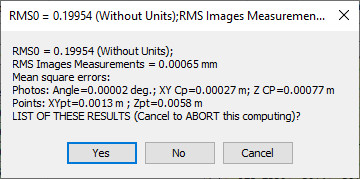
Listing AERO
All these root mean square errors are derived from the average of the Rms observed by topic. This in order to give a general idea of the quality of the aerotriangulation, without going through the entire listing.
Rms0: Mathematical value of the general root mean square error. From this value follow all the other root mean square errors, as well the distance Rmss as of the angle or of the plate measurement. If this value doubles, then all root mean square errors will double.
Rms Measurement Cliché: It is the root mean square error of all the deviations observed on the Images measurements
Rms Images (Angle, XY and Z): Mean squared error observed on the Phi, Omega and Kappa as well as on the XY and Z of the perspective centers of the Images.
Rms Points: Root mean square error on the XY and Z of the calculated points
AERO Listing
TrajectographyOffsets:
These values only appear if these values are active. They are then taken into account in the least squares calculation and enter as unknowns.
dX,dY dZ are the absolute values of the constants to be added to the coordinates of the trajectory GPS points in meters.
Roll,Pitch,Yaw Roll, Pitch,Yaw correction values to apply to the aircraft's inertial measurement. They affect the PHI, Omega and Kappa of the GPS CP angles
.
dX.Cam,dY.Cam correspond to the corrections to
to be made to the offset of the GPS X Ys in the system linked to the aircraft.
kX Image,kY Image correspond to the X and Y scale corrections on the measurements in the axis system of the Images
Listing AERO
Results of compensation calculation relative to each Clichés: XYZ and Omega, Phi, Kappa of the perspectival centers as well as their EMQ.
In the cases of a focal re-calculation, the "Focal" column is also filled in.
Listing AERO
Reminder of the XYZ and Omega, Phi, Kappa values of the GPS Points used for the
compensation in block. Insofar as these values are non-existent or not taken in the
taken in the calculation, they do not appear.
Listing AERO
We recall here the differences between the GPS points of the trajectography and the
perspectival centers from the calculation. These differences correspond to the subtraction
of the 2 upper lines corrected for GPS offsets if any.
Listing AERO
CteX,CteY,CteZ,CteOmega,CtePhi,CteKappa is the average of all
GPS deviations noted in (LA 05). This average allows us to see if it is
interesting to add a constant to these GPS data to improve the
project results.
We can then add these constants to a selection of Images using the menu
Right click on the list of Images, Tag <Images>
AERO Listing
Provided coordinates and compensated coordinates of field points. Their accuracy is provided in the form of Rms X, Y and Z as well as ellipses.
The grounds points that have a positive Rms are recalculated. The differences in XYZ
between the coordinates provided and the calculations are provided in the last 3
columns.
Listing AERO
Same as in (LA 07) for the Ties Points. As there are no
measured coordinates in the field, there are no discrepancies either.
Listing AERO
List of image measurements used for the calculation. They are sorted by Images.
Rms X, Rms Y: Rms in image units (mm) relating to each measurement. These Rmss are only a reminder of your entry.
You can change these values by a Right Click on a selection of snapshots in the tag.
Deviation X, Deviation Y: Deviations in unit Images (mm) between the measurement made and the intersection of the ray starting from the target point, passing through the perspective center with this Image.

You can view the tolerance ellipses related to the last calculation by clicking the button:
You will then be asked for a drawing scale and the Autocad Entities will be created.
Import export with market software handling of model files:
PMS3D Aerotriangulation data are stored in a xxx.model file.
It is an ASCII file totally open and readable by any professional. It can be manipulated with a text editor;
be manipulated with a text editor or a spreadsheet.
All information is readable and formatted to be easy to produce.
In addition, the software is the least demanding possible and if possible does its best to
to read what is readable, even partially, and to complete what is missing.
However, lines measures snapshots: "CLIMEA;6956;?5...." without previously line Creation
Cliché: "CLICHE;6955;\F..." will not be taken into account.
This property is actually interesting because, to clean up a
file xxx.model, it is enough to remove the lines of creation of clichés at the
the beginning of the file to read only the remaining snapshots (this is a simple filtering method
(This is a simple filtering method to implement). The best method is still to right-click on a selection of
on a selection of Images.
There are functions to purge unnecessary information (e.g. points not measured)
There are functions to purge unnecessary information (unmeasured points for example), to extract a part of the file (on a selection of
(on a selection of Images in a scrollbar or graphically in Autocad), to merge several
several files in overwrite or merge mode.
There is an import/export of PCI Geomatic .PRJ files.
There is an import and export of KLT data. In export, it is necessary to recalculate the
information provided on KLT.
There is import and export of graphic data xxxx.atl from KLT (KLT module of
conversion module xxx.atl to ASCII is required).
A KLT file arrives as a work AREA in Autocad.
It is necessary for this to establish a correspondence table.
Import and export of PCAP files from Zeiss.
Import of points (---.FIC) and cliché measurements from IGN.
Import of points and cliché measurements from the LEICA system.
Import and Export to BINGO which is read and written by almost all software.
Import and Export to INPHO products.
Import and Export to PHOTOSCAN
PMS3D works directly with the xxx.psz file generated by PHOTOSCAN.
These "psz" files are actually an assembly of XML, TIF, PLY and other files compatible with WinZip.
PMS3D works mainly on the DOC.XML file contained in this ".psz" file
In Import (PHOTOSCAN to PMS3D):
Menu : Files-Import-Photoscan Import
- The existing cameras of Pms3D are not modified, the others are imported. If you want to import a camera that is in the PMS3D file, rename it or destroy it before importing.
- Snapshots are created or merged depending on whether they exist or not
- The Grounds and Ties Points are merged with the existing ones
- It is possible to import the points correlated automatically by PHOTOSCAN.
These points are all named with the form ACPnnnnnn, nnnnnnn being the PHOTOSCAN index for this point
Points with this number in PMS3D are overwritten
In Export (PMS3D to PHOTOSCAN):
Menu : Files-Export-Photoscan Export
- The existing PHOTOSCAN cameras are modified if they exist, the others are created
- Snapshots are created or merged depending on whether they exist or not
- The Grounds and Ties Points are merged with the existing ones (The 'Markers')
- Measures overwrite existing measures if they Exist.
- Auto correlation points are not Exported
If you want to process a file using PHOTOSCAN and PMS3D, the recommended procedure is as follows:
PHOTOSCAN: insert and calculate their approximate orientations
PMS3D: Import the results and recalculate the Aerotriangulation en bloc if necessary
PMS3D : Create the Models
PMS3D: Ready for vector input
PMS3D : Export in PHOTOSCAN of the Aerotriangulation
PHOTOSCAN : PHOTOSCAN is ready to calculate the automatic DTM
Import and Export to Pix4dMapper
PMS3D works directly with the "xxx.p4d" files generated by Pix4dMapper.
These "p4d" files can be edited by any ASCII or XML editor.
The measurements on the correlated points are retrieved in the "../paramms/xxx_tp_bingo.txt" file. Only the pro version of Pix4dMapper generates this file
To ensure that the orientations and tuning elements are compatible, it is necessary to verify that in pix4d, "Optimization of internal parameters" is on "None".
This is accessed by: Local Processing-Options-AdvancedCalibration).
Translated with www.DeepL.com/Translator (free version)
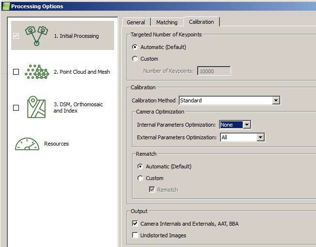
En import (Pix4dMapper vers PMS3D):
Menu : Fichiers-Importation-Importation PIX4D (.p4d)
L'importation peut être en ASCII ou en Binaire.
L'importation binaire est sensible à la version de pix4d.
- The existing cameras of Pms3d are not modified, the others are imported. If you want to import a camera that is in the PMS3D file, rename it or destroy it before importing.
- Snapshots are created or merged depending on whether they exist or not
- The Grounds and Ties Points are merged with the existing ones
- It is possible to import the points automatically correlated by Pix4dMapper.
In Export (PMS3D to Pix4dMapper):
Menu: Files-Export-Export PIX4D (.p4d)
- The existing Pix4dMapper cameras are modified if they exist, the others are created
- Snapshots are created or merged depending on whether they exist or not
- The Grounds and Ties Points are merged with the existing ones (The 'Markers')
- Measures overwrite existing measures if they Exist.
- Auto correlation points are not Exported
If you want to process a file using Pix4dMapper and PMS3D, the recommended procedure is as follows:
Pix4dMapper: insert and calculate their approximate orientations
PMS3D: Import the results and recalculate the Aerotriangulation in bulk if necessary
PMS3D : Create the Models
PMS3D: Ready for vector input
PMS3D : Export in Pix4dMapper of the Aerotriangulation
Pix4dMapper : Pix4dMapper is ready to calculate the automatic DTM and other
features
Export to PATB or PHOTOMOD
The best way to export PMS3D Aerotriangulation data to PHOTOMOD is to use the PATB Format.
This function creates the following files:
- NomCamera.x-cam: This file can be imported by PHOTOMOD or simply be copied into the "Camera" directory of your PHOTOMOD project.
- ProjectName.XYZ: It contains all the coordinates of the control points. There is no type or precision information.
- ProjectName.ORI: It contains all the information relating to the external orientations of the images (XYZ CP, Omega, Phi and Kappa) in the form of a matrix (4.3)
- ProjectName_mm.mea: It contains all the images measurements (in mm).
- NameProject_pix.mea : It contains all the clichés measurements (in pixel). In photomod, it is preferable to import this file rather than the one in mm.
Import of PATB files (LEICA LPS)
You must have mounted your project containing the images in this project.
You can import the files --.x-cam,--.XYZ, --.ORI, --.mea seen in export above.
You can select several of these files at the same time.
You will have to calculate the orientations Associate the cameras to the Images, calculate the internal orientations and mount the model.
Import of Aerotriangulation from native PHOTOMOD files
You can start from a Blank file, otherwise most of the data will be overwritten.
This function allows you to import the Native files from PHOTOMOD:
- "Images.x-ini": provides the Image names
- "Camera/*.x-cam": provides the list of cameras and their characteristics.
- "IntOr.x-ini": provides the list of Images and their associated camera.
- "ExtOr. x-ini" : provides the Orientations of the Images and the GPS points.
- "BundlePoints.x-ini" : provides the Land points, the Image Measurements.
- "BlockCT.x-ini" : provides the final orientations of the Images.
The fabrication of the Models remains to be done, see the chapter.
We are at your disposal to study the implementation of other formats.
Example of Aerotriangulation file ( *.PMS3D):
Example Listing from Block by Beam calculation
Display of the Aerotriangulation Imlages nbsp;
This Export Function is part of the Aerotriangulation module.
Command:PMS_AERO
This way you create INSERT with Attributes:
AENO = Cliché No. allowing the link with the AERO file ---.model
AEOINT = Internal Orientation Measurements
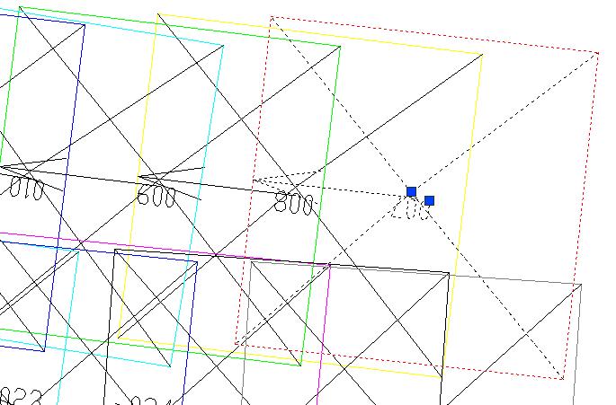
You can display the Images relating to these INSERTs by the Menu of the PMS3D palette:
or the command: PMS_IMGLOAD
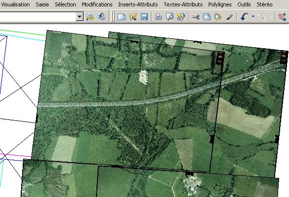
Aerotriangulation tools menu
Menu to change the coordinate system.
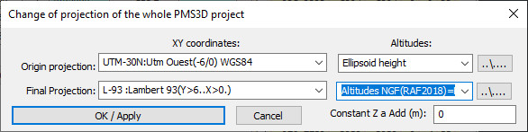
This function allows you to change the coordinate system of all the elements (points and angles) of the whole PMS3D project.
You have to define the starting system and the final system in planimetry and altimetry.
The definition of the ellipsoid elements, the datum shift and the list of projections can be found in the file '..\INI\Projections.INI' or '..\INI\Projections.DEF'.
You can define new ones if you wish.
You can define new ones if you wish.
For French projections, correction grids are used.
RAF98_BL.GRA" is an Altimetric correction grid to pass from the Heights
of the WGS84 (or GRS80) ellipsoid to NGF heights.
gr3df97a.txt" is an XY correction grid to switch from Lambert I, II, III
Lambert I, II, III... projections to Lambert 93 and Lambert 93 projections
Conic Conformal Zones 1 to 9.
There are 3 UTM 30 declared in the proposed version:
UTM-30:UTM West" (=UTM30N), the most common is based on
WGS84 ellipsoid, usually provided with an ellipsoid height.
"UTM-30ED50:UTM West" , on the Hayford ellipsoid with a datum shift of -87,-98,-121
"ED50_IGN" , identical to the previous one but with a datum shift of -84,-97,-117.
There are a multitude of projection systems. To avoid errors, try to work either in UTM WGS84 (or GRS80), or in Lambert 93 or Lambert
93 Zone for France.
To the extent that you have measured terrain points, applying an offset correction causes you to correct the
error residuals produced by this change in projection system; especially in Z.
Menu Import/Export GPS Snapshots and Perspective Centers.
This import function is identical to the one related to Images
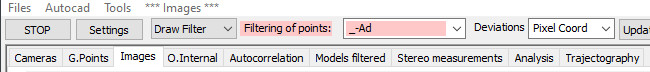
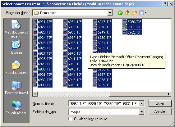
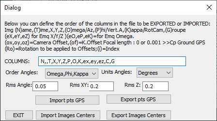 The X, Y, Z, Omega, Phi, Kappa data respect the classical conventions of photogrammetry.
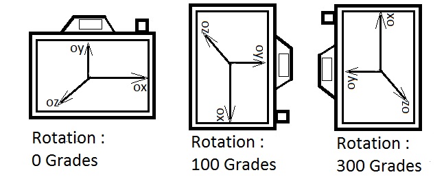
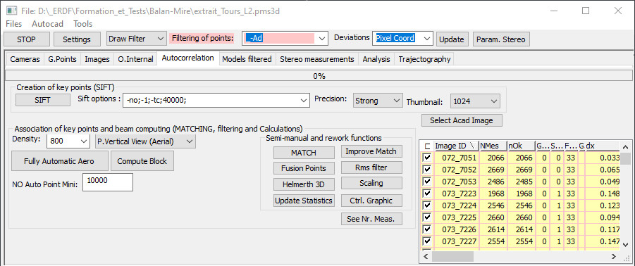
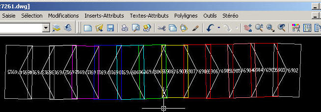
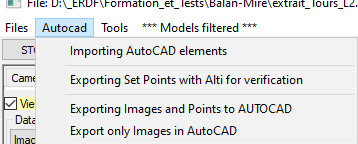
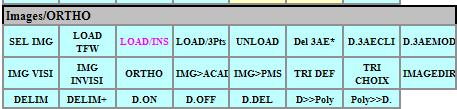
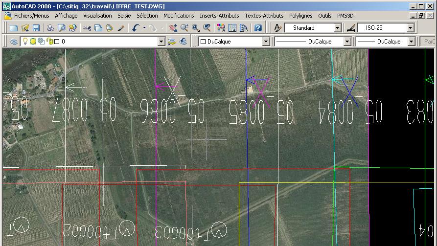
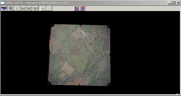
 you are conforming the unmapped plate to the mapped plate.
In the drop-down menu of point names validate AUTO*
(MS 01). The system will automatically move as close as possible to the points to be measured. You have a pedal (or button) to block
to lock one Image in relation to the other, another to launch the Zoom=2, and a third to validate the point.
a third to validate the point. The space bar skips the measurement of an unmeasurable or useless point.
you are conforming the unmapped plate to the mapped plate.
In the drop-down menu of point names validate AUTO*
(MS 01). The system will automatically move as close as possible to the points to be measured. You have a pedal (or button) to block
to lock one Image in relation to the other, another to launch the Zoom=2, and a third to validate the point.
a third to validate the point. The space bar skips the measurement of an unmeasurable or useless point.